テキストを書き込む場合も、画像と同じ要領です。
<?php
$short = '2018/02/26	Credit Suisse Securities	0.470%	-0.150%	42,700株	-13,300\n';

file_put_contents("sample.txt", $short);
?>
書き込まれました。
追加する場合は、第三引数にFILE_APPENDとします。
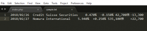
<?php

$short = "2018/02/27	Nomura International	5.940%	+0.250%	535,100株	+22,700\r\n";

file_put_contents("sample.txt", $short, FILE_APPEND);
?>
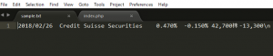
上手く追加されてますね。
ではテキストを配列で持っていた場合はどうでしょうか? foreachで回してみます。
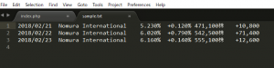
<?php
$short = array(
	"2018/02/21	Nomura International	5.230%	+0.120%	471,100株	+10,800\r\n",
	"2018/02/22	Nomura International	6.020%	+0.790%	542,500株	+71,400\r\n",
	"2018/02/23	Nomura International	6.160%	+0.140%	555,100株	+12,600\r\n"
	);
foreach($short as $value){
	file_put_contents("sample.txt", $value, FILE_APPEND);
}
?>
おおお、入ってますね。少し感動しました。