<?php
for ($i=0; $i<count($_FILES['files']['name']) and $i < 2; $i++) {
$file_ext = pathinfo($_FILES["files"]["name"][$i], PATHINFO_EXTENSION);
if (FileExtensionGetAllowUpload($file_ext) && is_uploaded_file($_FILES["files"]["tmp_name"][$i])) {
if(move_uploaded_file($_FILES["files"]["tmp_name"][$i], "upload/img/".$_FILES["files"]["name"][$i])) {
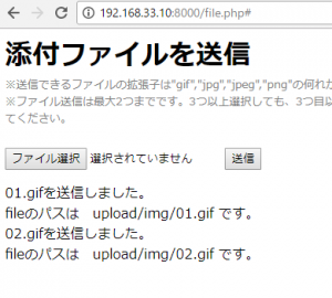
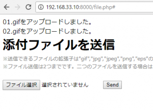
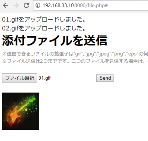
$message .= $_FILES["files"]["name"][$i] . "を送信しました。<br>";
$message .= "fileのパスは upload/img/".$_FILES["files"]["name"][$i]." です。<br>";
} else {
$message = "ファイルをアップロードできません。<br>";
}
} else {
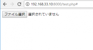
$message = "ファイルが選択されていません。<br>";
}
}
function FileExtensionGetAllowUpload($ext){
$allow_ext = array("gif","jpg","jpeg","png");
foreach($allow_ext as $v){
if ($v === $ext){
return 1;
}
}
return 0;
}
?>
<style>
.thumb {
height: 100px;
width: 100px;
border: 1px solid #000;
margin: 10px 5px 0 0;
}
h1 {
margin:0px;
}
#caution {
color:gray;
font-size:small;
}
</style>
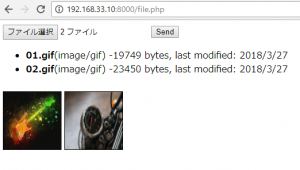
<h1>添付ファイルを送信</h1>
<div id="caution">
※送信できるファイルの拡張子は"gif","jpg","jpeg","png"の何れかです。<br>
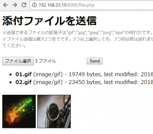
※ファイル送信は最大2つまでです。3つ以上選択しても、3つ目以降は送れません。また、二つのファイルを送信する場合は、キーボードの"ctl"ボタンなどで二つ選択した状態で開いてください。</div><br>
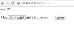
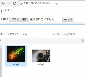
<form action="#" method="post" enctype="multipart/form-data">
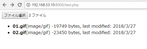
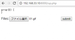
<input type="file" id="files" name="files[]" multiple />
<input type="submit" value="送信">
</form>
<?php echo $message; ?>
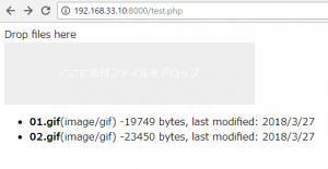
<output id="list"></output>
<script>
function handleFileSelect(evt){
var files = evt.target.files;
if(files.length > 2){
files = files.slice(0, 2);
}
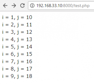
for (var i = 0, f; f = files[i]; i++) {
// for (var i = 0, f; f = files[i]; i++) {
if (!f.type.match('image.*')) {
continue;
}
var reader = new FileReader();
reader.onload = (function(theFile){
return function(e){
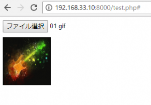
var span = document.createElement('span');
span.innerHTML = ['<img class="thumb" src="', e.target.result,
'" title="', escape(theFile.name), '"/>'].join('');
document.getElementById('list').insertBefore(span, null);
};
})(f);
reader.readAsDataURL(f);
}
var output = [];
for (var i = 0, f; f = files[i]; i++) {
// for (var i = 0, f; f = files[i]; i++) {
output.push('<li><strong>', escape(f.name), '</strong> (', f.type || 'n/a', ') - ',
f.size, ' bytes, last modified: ',
f.lastModifiedDate.toLocaleDateString(), '</li>');
}
document.getElementById('list').innerHTML = '<ul>' + output.join('') + '</ul>';
}
document.getElementById('files').addEventListener('change', handleFileSelect, false);
</script>
同じファイル名を送信すると、ファイルが上書きされてしまうので、保存するディレクトリを送信ごとにユニークにする必要がありますね。