
$git push
Local(master) to Remoto(origin) repository
Hosting on GitHub
Now the problem with GitHub is that the name is so similar to Git that people sometimes conflate Git and GitHub and think they’re the same thing when they’re actually quite different.
-Git is a version control tool
-GitHub is a service to host Git projects
https://git-scm.com/book/en/v2/Git-Basics-Working-with-Remotes#_showing_your_remotes
git commit
[vagrant@localhost my-travel-plans]$ git add README.md
[vagrant@localhost my-travel-plans]$ git commit -m “first commit”
[master (root-commit) e226c9a] first commit
1 file changed, 2 insertions(+)
create mode 100644 README.md
[vagrant@localhost my-travel-plans]$ git status
On branch master
Untracked files:
(use “git add
app.css
index.html
nothing added to commit but untracked files present (use “git add” to track)
[vagrant@localhost my-travel-plans]$ git commit -am “second commit”
On branch master
Untracked files:
app.css
index.html
nothing added to commit but untracked files present
[vagrant@localhost my-travel-plans]$ git add app.css
[vagrant@localhost my-travel-plans]$ git add index.html
[vagrant@localhost my-travel-plans]$ git commit -m “second commit”
[master f5e2913] second commit
2 files changed, 77 insertions(+)
create mode 100644 app.css
create mode 100644 index.html
[vagrant@localhost my-travel-plans]$ git status
On branch master
nothing to commit, working directory clean
Add a remote repository
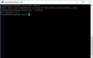
[vagrant@localhost git]$ git remote
fatal: Not a git repository (or any of the parent directories): .git
[vagrant@localhost git]$ git --version
git version 2.2.1
create a new directory with the name my-travel-plans
use git init to turn the my-travel-plans directory into a Git repository
create a README.md file
create index.html
create app.css
README.md
# Travel Destinations
A simple app to keep track of destinations I'd like to visit.
index.html
<!doctype html>
<html lang="en">
<head>
<meta charsete="utf-8">
<title>Travels</title>
<meta name="description" content="">
<link rel="stylesheet" href="css/app.css">
</head>
<body>
<div class="container">
<div class="destination-container">
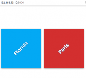
<div class="destination" id="florida">
<h2>Florida</h2>
</div>
<div class="destination" id="paris">
<h2>Paris</h2>
</div>
</div>
</div>
</html>
app.css
html {
  box-sizing: border-box;
  height: 100%;
}

*,
*::before,
*::after {
  box-sizing: inherit;
}

body {
  display: flex;
  margin: 0;
  height: 100%;
}

.container {
  margin: auto;
  padding: 1em;
  width: 80%;
}

.destination-container {
  display: flex;
  flex-flow: wrap;
  justify-content: center;
}

.destination {
  background: #03a9f4;
  box-shadow: 0 1px 9px 0 rgba(0, 0, 0, 0.4);
  color: white;
  margin: 0.5em;
  min-height: 200px;
  flex: 0 1 200px;
  display: flex;
  justify-content: center;
  align-items: center;
  text-align: center;
}

h2 {
  margin: 0;
  transform: rotate(-45deg);
  text-shadow: 0 0 5px #01579b;
}

#florida {
  background-color: #03a9f4;
}

#paris {
  background-color: #d32f2f;
}
Git intro
creating repositories with git init and git clone
reviewing repos with git status
using git log and git show to review past commits
being able to make commits with git add
commit them to the repo with git commit
need to know about branching, merging branches together, and resolving merge conflicts
being able to undo things in Git:
git commit –amend to undo the most recent commit or to change the wording of the commit message
git reset if you’re comfortable with all of these, then you’ll be good to go for this
It’s incredibly helpful to make all of your commits on descriptively named topic branches. Branches help isolate unrelated changes from each other.
So when you’re collaborating with other developers make sure to create a new branch that has a descriptive name that describes what changes it contains.
git remote
git push
git pull
Git is a distributed version control system which means there is not one main repository of information. Each developer has a copy of the repository. So you can have a copy of the repository (which includes the published commits and version history) and your friend can also have a copy of the same repository. Each repository has the exact same information that the other ones have, there’s no one repository that’s the main one.
The way we can interact and control a remote repository is through the Git remote command:
$ git remote
Alpha and Jitter
'''(r)
ggplot(aes(x = age, y = friends_initiated), data = pf)
 geom_point(alpha = 1/10, position = 'jitter')
'''
age_groups <- group_by(pf, age)
pf.fc_by_age <- summarise(age_groups,
	friend_count_mean = mean(friend_count),
	friend_count_median = median(friend_count),
	n = n())
pf.fc_by_age <- arrange(pf.fc_by_age, age)
head(pf.fc_by_age)
Explore Variables
Scatterplots
'''(r)
library(ggplot2)
pf <- read.csv('pseudo_facebook.tsv', sep = '\t')

qplot(x = age, y = friend_count, data = pf)
qplot(age, friend_count, data = pf)
'''
'''(r)
qplot(x = age, y = friend_count, data = pf)

ggplot(aes(x = age, y= friend_count), data = pf) + geom_point()

summary(pf$age)
'''
'''(r)
ggplot(aes(x = age, y = friend_count),data = pf)+
	geom_point(alpha = 1/20) + xlim(13, 90)
'''
Histogram of Users’ birth
'''(r)
install.packages('ggplot2')

names(pf)
qplot(x -dob_day, data - pf)
'''
'''(r)
qplot(x - friend_count, data - pf)
'''
'''(r)
qplot(x - friend_count, data - pf, xlim - c(0, 1000))

qplot(x - friend_count, data_pf) +
	scale_x_continuous(limits - c(0, 1000))
'''
R Markdown Documents
'''{r}
# the hash or pound symbol inside the block creates
# a comment. These three lines of are not code and cannot be
x <- [1:10]
mean(x)
'''
a <- c(1,2,5.3,6,-2,4) # numeric vector
b <- c("one","two","three") # character vector
c <- c(TRUE,TRUE,TRUE,FALSE,TRUE,FALSE) #logical vector
reddit <- read.csv('reddit.csv')

table(reddit$employment)

str(reddit)
levels(reddit$age.range)

library(ggplot2)
qplot(data = reddit, x = age.range)
Markdown Cheatsheet
https://github.com/adam-p/markdown-here/wiki/Markdown-Cheatsheet