https://developers.google.com/youtube/v3/getting-started?hl=ja
Youtube apiを使うには、cloud consoleで、プロジェクトの登録が必要となります。
https://console.developers.google.com/projectcreate
新しいプロジェクトを作りましょう。
ここでは、nameは[youtube-app]とします。
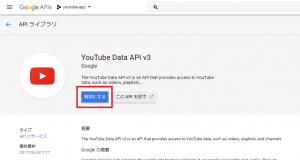
そして、サービスからYouTube Data API(v3)を有効にします。
リソースの種類
activity, channel, channelBanner, playlist, playlistItem, search result, subscription, thumbnail, video, videoCategory
操作
list: リソースのリストをGET
insert: 新しいリソースをPOST
update: 既存のリソースをPUT
delete: リソースをDELETE
サポートされる操作
activity, caption, channel, channelBanner, channelSection, comment, commentThread, guideCategory, i18nLanguage, i18nRegion, playlist, playlistItem, search result, subscription, thumbnail, video, videoCategory, watermark
partパラメーター:リソースを取得する API リクエストまたはリソースを返す API リクエストに対して必須のパラメータ。API レスポンスに含める必要がある 1 つ以上の最上位レベルのリソース プロパティを指定。
fieldsパラメーター:fields パラメータは API レスポンスをフィルタリングし、part パラメータ値で指定されたリソース パーツだけが含まれるようにする。
