つくってる人凄すぎてコーディングが嫌になるな。。
<!DOCTYPE html>
<html>
<head>
<title>Simple Map</title>
<meta name="viewport" content="initial-scale=1.0">
<meta charset="utf-8">
<style>
#map {
height: 50%;
margin-top: 10px;
}
html, body {
height: 100%;
margin: 10px;
padding: 0;
}
</style>
</head>
<body>
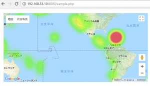
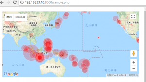
<div id="map"></div>
<script>
var map;
function initMap() {
map = new google.maps.Map(document.getElementById('map'), {
zoom: 2,
center: {lat: -33.865427, lng: 151.196123},
mapTypeId: 'terrain'
});
var script = document.createElement('script');
script.src = 'https://developers.google.com/maps/documentation/javascript/examples/json/earthquake_GeoJSONP.js';
document.getElementsByTagName('head')[0].appendChild(script);
}
function eqfeed_callback(results) {
var heatmapData = [];
for (var i = 0; i < results.features.length; i++) {
var coords = results.features[i].geometry.coordinates;
var latLng = new google.maps.LatLng(coords[1], coords[0]);
heatmapData.push(latLng);
}
var heatmap = new google.maps.visualization.HeatmapLayer({
data: heatmapData,
dissipating: false,
map: map
});
}
// // window.eqfeed_callback = function(results) {
// // for (var i = 0; i < results.features.length; i++) {
// // var coords = results.features[i].geometry.coordinates;
// // var latLng = new google.maps.LatLng(coords[1],coords[0]);
// // var marker = new google.maps.Marker({
// // position: latLng,
// // map: map
// // });
// // }
// }
</script>
<script async defer
src="https://maps.googleapis.com/maps/api/js?key=hoge&libraries=visualization&callback=initMap">
</script>
</body>
</html>