
ガウス関数は正規分布関数
a exp{-(x-b)^2 / 2C^2}
こちらもガウス関数の一種
1/√2πσ exp (- (x – μ)^2 / 2σ^2)
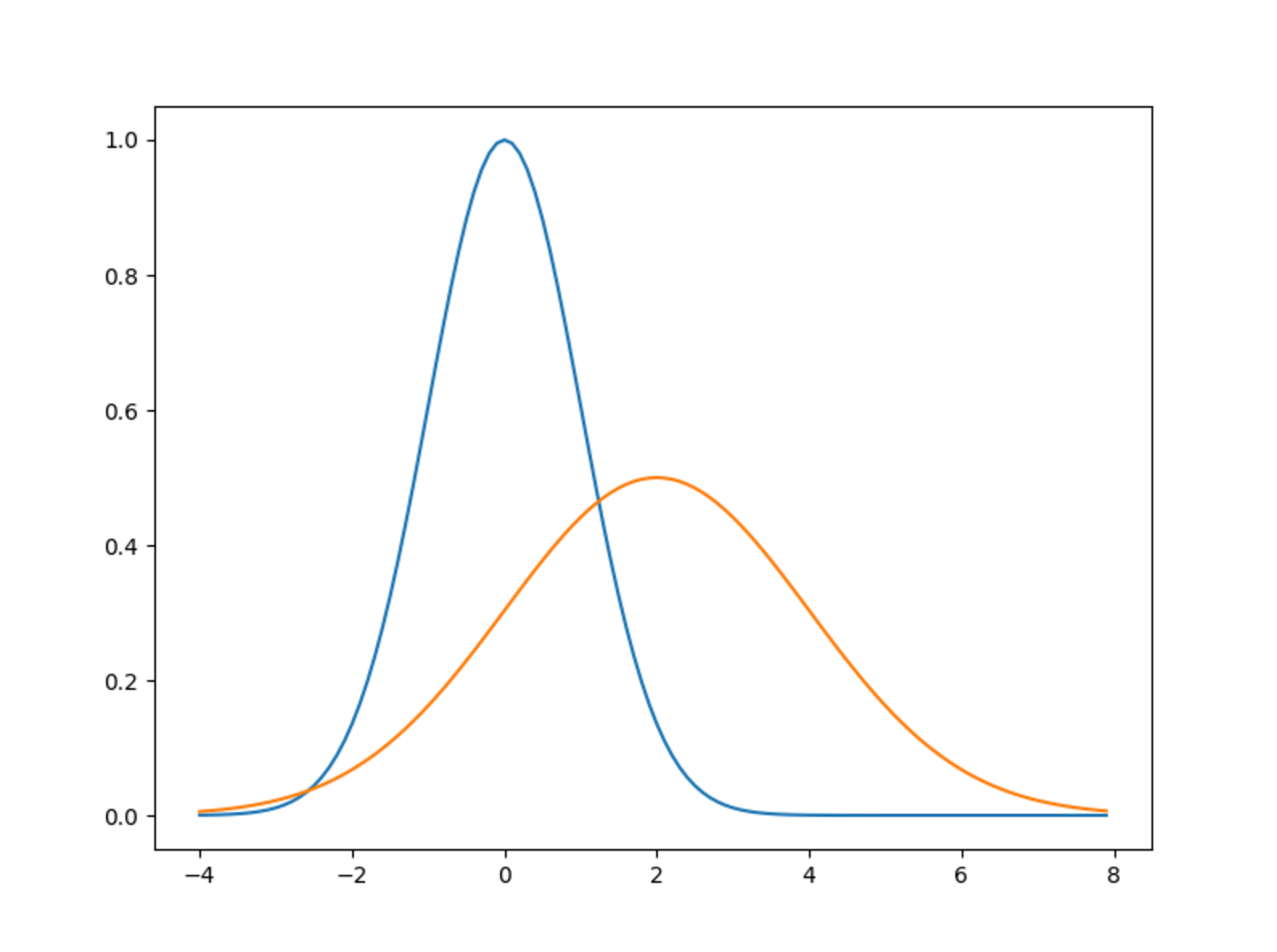
import numpy as np
import matplotlib.pylab as plt

def gauss(x, a = 1, mu = 0, sigma = 1):
	return a * np.exp(-(x - mu)**2 / (2*sigma**2))

fig = plt.figure(figsize = (8, 6))
ax = fig.add_subplot(111)

x = np.arange(-4, 8, 0.1)
f1 = gauss(x)
f2 = gauss(x, a = 0.5, mu=2, sigma= 2)

ax.plot(x, f1)
ax.plot(x, f2)
正規分布になってますね。
ガウス分布の微分は
– (x – μ)/√2πσ^3 (- (x – μ)^2 / 2σ^2) です。