
unwanted = nltk.corpus.stopwords.words("english")
unwanted.extend([w.lower() for w in nltk.corpus.names.words()])

def skip_unwanted(pos_tuple):
	word, tag = pos_tuple
	if not word.isalpha() or word in unwanted:
		return False
	if tag.startswith("NN"):
		return False
	return True

positive_words = [word for word, tag in filter(
	skip_unwanted,
	nltk.pos_tag(nltk.corpus.movie_reviews.words(categories=["pos"]))
)]
negative_words = [word for word, tag in filter(
	skip_unwanted,
	nltk.pos_tag(nltk.corpus.movie_reviews.words(categories=["neg"]))
)]

positive_fd = nltk.FreqDist(positive_words)
negative_fd = nltk.FreqDist(negative_words)

common_set = set(positive_fd).intersection(negative_fd)

for word in common_set:
	del positive_fd[word]
	del negative_fd[word]

top_100_positive = {word for word, count in positive_fd.most_common(100)}
top_100_negative = {word for word, count in negative_fd.most_common(100)}

unwanted = nltk.corpus.stopwords.words("english")
unwanted.extend([w.lower() for w in nltk.corpus.names.words()])

positive_bigram_finder = nltk.collocations.BigramCollocationFinder.from_words([
	w for w in nltk.corpus.movie_reviews.words(categories=["pos"])
	if w.isalpha() and w not in unwanted
])

negative_bigram_finder = nltk.collocations.BigramCollocationFinder.from_words([
	w for w in nltk.corpus.movie_reviews.words(categories=["neg"])
Category: Natural Language
[NLTK] sentiment analysis
NLTK has a built-in pretrained sentiment analyzer, VADER(Valence Aware Dictionary and sEntiment Reasoner)
import nltk
from pprint import pprint
from nltk.sentiment import SentimentIntensityAnalyzer

sia = SentimentIntensityAnalyzer()
pprint(sia.polarity_scores("Wow, NLTK is really powerful!"))
$ python3 app.py
{‘compound’: 0.8012, ‘neg’: 0.0, ‘neu’: 0.295, ‘pos’: 0.705}
compoundはaverageで-1から1までを示す
twitter corpus
tweets = [t.replace("://", "//") for t in nltk.corpus.twitter_samples.strings()]

def is_positive(tweet: str) -> bool:
    """True if tweet has positive compound sentiment, False otherwise."""
    return sia.polarity_scores(tweet)["compound"] > 0

shuffle(tweets)
for tweet in tweets[:10]:
    print(">", is_positive(tweet), tweet)
$ python3 app.py
> False Most Tory voters not concerned which benefits Tories will cut. Benefits don’t figure in the lives if most Tory voters. #Labour #NHS #carers
> False .@uberuk you cancelled my ice cream uber order. Everyone else in the office got it but me. 🙁
> False oh no i’m too early 🙁
> False I don’t know what I’m doing for #BlockJam at all since my schedule’s just whacked right now 🙁
> False What should i do .
BAD VS PARTY AGAIN :(((((((
> True @Shadypenguinn take care! 🙂
> True Thanks to amazing 4000 Followers on Instagram
If you´re not among them yet,
feel free to connect :-)… http//t.co/ILy03AtJ83
> False RT @mac123_m: Ed Miliband has spelt it out again. No deals with the SNP.
There’s a choice:
Vote SNP get Tories
Vote LAB and get LAB http//…
> True @gus33000 but Disk Management is same since NT4 iirc 😀
Also, what UX refinements were in zdps?
> False RT @KevinJPringle: One of many bizarre things about @Ed_Miliband’s anti-SNP stance is he doesn’t reject deal with LibDems, who imposed aust…
postivie_review_ids = nltk.corpus.movie_reviews.fileids(categories=["pos"])
negative_review_ids = nltk.corpus.movie_reviews.fileids(categories=["neg"])
all_review_ids = positive_review_ids + negative_review_ids

def is_positive(review_id: str) -> bool:
	"""True if the average of all sentence compound scores is positive. """
	text = nltk.corpus.movie_reviews.raw(review_id)
	scores = [
		sia.polarity_scores(sentence)["compound"]
		for sentence in nltk.sent_tokenize(text)
	]
	return mean(scores) > 0

shuffle(all_review_ids)
correct = 0
for review_id in all_review_ids:
	if is_positive(review_id):
		if review in positive_review_ids:
			correct += 1
	else:
		if review in negative_review_ids:
			correct += 1

print(F"{correct / len(all_review_ids):.2%} correct")
既にcorpusがあるのは良いですね。
[NLTK] Word frequency
$ pip3 install nltk
### download
NLTK can be download resouces
– names, stopwords, state_union, twitter_samples, moview_review, averaged_perceptron_tagger, vader_lexicon, punkt
import nltk

nltk.download([
	"names",
	"stopwords",
	"state_union",
	"twitter_samples",
	"movie_reviews",
	"averaged_perceptron_tagger",
	"vader_lexicon",
	"punkt",
])
State of union corpus
words = [w for w in nltk.corpus.state_union.words() if w.isalpha()]
to use stop words
words = [w for w in nltk.corpus.state_union.words() if w.isalpha()]
stopwords = nltk.corpus.stopwords.words("english")
words = [w for w in words if w.lower() not in stopwords]
word_tokenize()
text = """
For some quick analysis, creating a corpus could be overkill.
If all you need is a word list,
there are simpler ways to achieve that goal.
"""
pprint(nltk.word_tokenize(text), width=79, compact=True)
most common
fd = nltk.FreqDist(words)
pprint(fd.most_common(3))
$ python3 app.py
[(‘must’, 1568), (‘people’, 1291), (‘world’, 1128)]
specific word
fd = nltk.FreqDist(words)
pprint(fd["America"])
$ python3 app.py
1076
### concordance
どこに出現するかを示す
text = nltk.Text(nltk.corpus.state_union.words())
text.concordance("america", lines=5)
$ python3 app.py
Displaying 5 of 1079 matches:
would want us to do . That is what America will do . So much blood has already
ay , the entire world is looking to America for enlightened leadership to peace
beyond any shadow of a doubt , that America will continue the fight for freedom
to make complete victory certain , America will never become a party to any pl
nly in law and in justice . Here in America , we have labored long and hard to
text = nltk.Text(nltk.corpus.state_union.words())
concordance_list = text.concordance_list("america", lines=2)
for entry in concordance_list:
	print(entry.line)
$ python3 app.py
would want us to do . That is what America will do . So much blood has already
ay , the entire world is looking to America for enlightened leadership to peace
other frequency distribution
words: list[str] = nltk.word_tokenize(
"""Beautiful is better than ugly.
Explicit is better than implicit.
Simple is better than complex.""")
text = nltk.Text(words)
fd = text.vocab()
fd.tabulate(3)
collocation
words = [w for w in nltk.corpus.state_union.words() if w.isalpha()]
finder = nltk.collocations.TrigramCollocationFinder.from_words(words)

pprint(finder.ngram_fd.most_common(2))
pprint(finder.ngram_fd.tabulate(2))
$ python3 app.py
[((‘the’, ‘United’, ‘States’), 294), ((‘the’, ‘American’, ‘people’), 185)]
(‘the’, ‘United’, ‘States’) (‘the’, ‘American’, ‘people’)
294 185
nltkが強力なのはわかった。
【株式投資】twitterで買い煽り・売り煽りが多いかpython・MeCabで調べる
優秀なトレーダーで、買い煽りが多いか、売り煽りが多いか、定性的に調べたいと思う方も多いだろう。というのも、「買い煽り」「売り煽り」というのは、ポジションを持ったイナゴの心理状態をかなり表しているからだ。当然、株が上がって欲しい時は買い煽りをするし、株価が下落して欲しい時は夢中で売り煽りを行う。外野から見たらやや滑稽に見えるかもしれないが、本人にとってはいたって真剣に行っている。なぜなら、案外、この煽りに影響を受けて売買をする人が多いからだ。話がややズレたが、したがって「買い煽り」「売り煽り」を定性的に分析さえできれば、より冷静に判断することができるので、株式投資のパフォーマンスは飛躍的に向上すると期待できる。そこで、本投稿では、Pythonを使って、買い煽り・売り煽り分析を行う。
yahooファイナンスの掲示板で調べたかったが、スクレイピングが禁止なので、twitterで銘柄コードと一緒につぶやかれている内容で、買い煽りが多いか、売り煽りが多いかを調べる。
自然言語処理の感情分析で極めて重要なのはガゼッタ(辞書)であろう。
東工大の高村教授が作成したPN Tableや東北大学の乾・岡崎研究室の日本語評価極性辞書が有名だが、買い煽り・売り煽りとは全く関係ないだろう。そのため、自分で辞書を作る必要がある。検討を重ね、以下の単語が入ってれば、それぞれ買い煽りのツイート、売り煽りのツイートとして評価することにした。
### 買い煽りのガゼッタ
‘買い’,’買う’,’特買い’,’安い’,’全力’,’爆益’,’ノンホル’,’超絶’,’本物’,’成長’,’反転’,’拾う’,’ホールド’,’踏み上げ’,’国策’,’ストップ高’,’上がる’,’初動’,’クジラ’,’売り豚’,’売り方’,’ハイカラ’,’頑張れ’,’貸借’,’反転’,’応援’,’強い’,’逆日歩’
### 売り煽りのガゼッタ
‘売り’,’売る’,’下がる’,’大損’,’ナイアガラ’,’ガラ’,’ジェットコースター’,’ダメ’,’嵌め込み’,’養分’,’退場’,’追証’,’赤字’,’ワラント’,’仕手’,’特売り’,’高い’,’アホルダー’,’イナゴ’,’撤退’,’倒産’,”,’買い豚’,’買い方’,’信用買’,’逃げろ’,’疑義’,’空売り’,’利確’,’損切’,’振い落とし’
### 銘柄に関連した呟きを取得
– tweepyで取得してテキストデータとして保存する
import tweepy
import datetime
import re

keyword = "6343 -RT"
dfile = "test.txt"

jsttime = datetime.timedelta(hours=9)

Consumer_key = ''
Consumer_secret = ''
Access_token = ''
Access_secret = ''

auth = tweepy.OAuthHandler(Consumer_key, Consumer_secret)
auth.set_access_token(Access_token, Access_secret)

api = tweepy.API(auth, wait_on_rate_limit = True)

q = keyword

tweets_data = []


for tweet in tweepy.Cursor(api.search, q=q, count=5,tweet_mode='extended').items(200):
	tweets_data.append(tweet.full_text + '\n')

fname = r"'" + dfile + "'"
fname = fname.replace("'", "")

with open(fname, "w", encoding="utf-8") as f:
    f.writelines(tweets_data)
### スコア分類
– つぶやきをMecabで形態素解析を行う
– 買い煽りのガゼッタのワードがつぶやかれたら買い煽り+1ポイント、売り煽りのガゼッタのワードがつぶやかれたら売り煽り+1ポイントとして評価した。
import MeCab

dfile = "test.txt"

fname = r"'" + dfile + "'"
fname = fname.replace("'","")

mecab = MeCab.Tagger("-Owakati")

words = []

with open(fname, 'r', encoding="utf-8") as f:

    reader = f.readline()

    while reader:

        node = mecab.parseToNode(reader)

        while node:
            word_type = node.feature.split(",")[0]
            if word_type in ["名詞", "動詞", "形容詞", "副詞"]:
                words.append(node.surface)
            node = node.next
        reader = f.readline()


# 買い煽りのgazetteer
buying_set = set(['買い','買う','特買い','安い','全力','爆益','ノンホル','超絶','本物','成長','反転','拾う','ホールド','踏み上げ','国策','ストップ高','上がる','初動','クジラ','売り豚','売り方','ハイカラ','頑張れ','貸借','反転','応援','強い','逆日歩'])

# 売り煽りのgazetter
selling_set = set(['売り','売る','下がる','大損','ナイアガラ','ガラ','ジェットコースター','ダメ','嵌め込み','養分','退場','追証','赤字','ワラント','仕手','特売り','高い','アホルダー','イナゴ','撤退','倒産','','買い豚','買い方','信用買','逃げろ','疑義','空売り','利確','損切','振い落とし'])

def classify_category(text):

	buying_score = 0
	selling_score = 0

	for ele in words:
		element = ele.split("\t")
		if element[0] == "EOS":
			break

		surface = element[0]

		if surface in buying_set:
			buying_score += 1
		if surface in selling_set:
			selling_score += 1

	print("買い煽りスコア:" + str(buying_score))
	print("売り煽りスコア:" + str(selling_score))

classify_category(words)
今回は、先日の金曜日にストップ高をつけたフリージア・マクロス(6343)で調べた。
$ python3 app.py
買い煽りスコア:13
売り煽りスコア:0
結果、買い煽りだらけとなった。
空売りを入れよう。
CornellのsentimentデータでTextClassification
### dataset
Cornell Natural Language Processing Groupの映画レビューのデータセットを使います。
http://www.cs.cornell.edu/people/pabo/movie-review-data/review_polarity.tar.gz
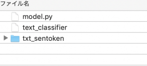
txt_sentokenフォルダ配下にnegativeとpositiveのデータが入っています。
### Sentiment Analysis with Scikit-Learn
1. import libraries and dataset
2. text preprocessing
3. converting text to numbers
4. training and test sets
5. training text classification model and predicting sentiment
6. evaluating the model
7. saving and loading the model
import numpy as np
import re
import nltk
from sklearn.datasets import load_files
nltk.download('stopwords')
import pickle
import nltk
nltk.download('wordnet')
from nltk.corpus import stopwords
from nltk.stem import WordNetLemmatizer
from sklearn.feature_extraction.text import CountVectorizer
from sklearn.feature_extraction.text import TfidfTransformer
from sklearn.model_selection import train_test_split
from sklearn.ensemble import RandomForestClassifier
from sklearn.metrics import classification_report, confusion_matrix, accuracy_score

# データ取得
movie_data = load_files("txt_sentoken")
X, y = movie_data.data, movie_data.target

# remove all the special characters
stemmer = WordNetLemmatizer()

documents = []

for sen in range(0, len(X)):
	# remove all the special character
	document = re.sub(r'\W', ' ', str(X[sen]))
	# remove all the single character
	document = re.sub(r'\s+[a-zA-Z]\s+', ' ', document)
	# remove all the single character from the start
	document = re.sub(r'\^[a-zA-Z]\s+', ' ', document)
	# substituting multiple spaces with single space
	document = re.sub(r'\s+', ' ', document, flags=re.I)
	# Removing prefixed 'b'
	document = re.sub(r'^b\s+', '', document)
	# converting to lowercase
	document = document.lower()
	# lemmatization (見出し語に変換)
	document = document.split()

	document = [stemmer.lemmatize(word) for word in document]
	document = ' '.join(document)

	documents.append(document)

# Bag of wordsとWord Embedding があるがここではBag of wordsを使う
# max_featuresはmost occuring world of 1500, min_dfはminimum number of documents contain this feature, max_dfはfraction corresponds to a percentage 最大70%
vectorizer = CountVectorizer(max_features=1500, min_df=5, max_df=0.7, stop_words=stopwords.words('english'))
# fit_transformでnumeric featuresに変換
X = vectorizer.fit_transform(documents).toarray()
# tfidf
tfidfconverter = TfidfTransformer()
X = tfidfconverter.fit_transform(X).toarray()

# training and testing sets
X_train, X_test, y_train, y_test = train_test_split(X, y, test_size=0.2, random_state=0)

# random forest algorithm, predicting sentiment
classifier = RandomForestClassifier(n_estimators=1000, random_state=0)
classifier.fit(X_train, y_train)

y_pred = classifier.predict(X_test)

print(confusion_matrix(y_test, y_pred))
print(classification_report(y_test, y_pred))
print(accuracy_score(y_test, y_pred))
$ python3 model.py
[[180 28]
[ 30 162]]
precision recall f1-score support
0 0.86 0.87 0.86 208
1 0.85 0.84 0.85 192
accuracy 0.85 400
macro avg 0.85 0.85 0.85 400
weighted avg 0.85 0.85 0.85 400
0.855
# save model
with open('text_classifier', 'wb') as picklefile:
    pickle.dump(classifier,picklefile)
import pickle
from sklearn.metrics import classification_report, confusion_matrix, accuracy_score

with open('text_classifier', 'rb') as training_model:
	model = pickle.load(training_model)

y_pred2 = model.predict(X_test)

print(confusion_matrix(y_test, y_pred))
print(classification_report(y_test, y_pred))
print(accuracy_score(y_test, y_pred))
Scikit-Learnでやるんやな。
Keras x CNN(Convolutional Neural Network)を試す
Convents have revolutionized image classification and computer vision to extract features from images.
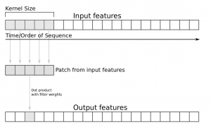
Keras use Conv1D layer
model = Sequential()
model.add(layers.Embedding(vocab_size, embedding_dim, input_length=maxlen))
model.add(layers.Conv1D(128, 5, activation='relu'))
model.add(layers.GlobalMaxPooling1D())
model.add(layers.Dense(10, activation='relu'))
model.add(layers.Dense(1, activation='sigmoid'))
model.compile(optimizer='adam',
			loss='binary_crossentropy',
			metrics=['accuracy'])
print(model.summary())
Model: “sequential”
_________________________________________________________________
Layer (type) Output Shape Param #
=================================================================
embedding (Embedding) (None, 100, 100) 100
_________________________________________________________________
conv1d (Conv1D) (None, 96, 128) 64128
_________________________________________________________________
global_max_pooling1d (Global (None, 128) 0
_________________________________________________________________
dense (Dense) (None, 10) 1290
_________________________________________________________________
dense_1 (Dense) (None, 1) 11
=================================================================
Total params: 65,529
Trainable params: 65,529
Non-trainable params: 0
_________________________________________________________________
KerasのSequentialモデルで、GloVeのPretrained Word Embeddingsを使ってみる
– Word2Vec developed by Google and GloVe, Stanford NLP Group
L co-occurrence matrix and matrix factorization
### Pretrained word embeddings
Global Vectors for Word RepresentationのサイトからはDLできないので、kaggleからDLします。
GloVe
e.g. 50 characters in first lines
$ head -n 1 glove.6B.50d.txt | cut -c-50
the 0.418 0.24968 -0.41242 0.1217 0.34527 -0.04445
import numpy as np
from keras.preprocessing.text import Tokenizer

def create_embedding_matrix(filepath, word_index, embedding_dim):
	global vocab_size
	vocab_size = len(word_index) + 1 # Adding 1 because of reserved 0 index
	embedding_matrix = np.zeros((vocab_size, embedding_dim))

	with open(filepath) as f:
		for line in f:
			word, *vector = line.split()
			if word in word_index:
				idx = word_index[word]
				embedding_matrix[idx] = np.array(
					vector, dtype=np.float32)[:embedding_dim]

	return embedding_matrix

tokenizer = Tokenizer(num_words=5000)
embedding_dim = 50
embedding_matrix = create_embedding_matrix(
	'glove.6B.50d.txt',
	tokenizer.word_index, embedding_dim)

nonzero_elements = np.count_nonzero(np.count_nonzero(embedding_matrix, axis=1))
print(nonzero_elements / vocab_size)
$ python3 glove.py
0.0
ん? 何かおかしい。。。
GlobalMaxPool1D layer
from keras.models import Sequential
from keras import layers

// 省略
vocab_size = len(tokenizer.word_index) + 1
embedding_dim = 50
maxlen = 100

model = Sequential()
model.add(layers.Embedding(vocab_size, embedding_dim,
							weights=[embedding_matrix],
							input_length=maxlen,
							trainable=False))
model.add(layers.GlobalMaxPool1D())
model.add(layers.Dense(10, activation='relu'))
model.add(layers.Dense(1, activation='sigmoid'))
model.compile(optimizer='adam',
			loss='binary_crossentropy',
			metrics=['accuracy'])
print(model.summary())
_________________________________________________________________
Layer (type) Output Shape Param #
=================================================================
embedding (Embedding) (None, 100, 50) 50
_________________________________________________________________
global_max_pooling1d (Global (None, 50) 0
_________________________________________________________________
dense (Dense) (None, 10) 510
_________________________________________________________________
dense_1 (Dense) (None, 1) 11
=================================================================
Total params: 571
Trainable params: 521
Non-trainable params: 50
_________________________________________________________________
None
なんかoutputが違うな
Keras Embedding Layer
keras parameter
– input_dim: the size of the vocabulary
– output_dim: the size of the dense vector
– input_length: the length of the sequence
from keras.preprocessing.text import Tokenizer
from keras.preprocessing.sequence import pad_sequences

// 省略
tokenizer = Tokenizer(num_words=5000)
tokenizer.fit_on_texts(sentences_train)

X_train = tokenizer.texts_to_sequences(sentences_train)
X_test = tokenizer.texts_to_sequences(sentences_test)

vocab_size = len(tokenizer.word_index) + 1
embedding_dim = 50
maxlen = 100

model = Sequential()
model.add(layers.Embedding(input_dim=vocab_size,
                            output_dim=embedding_dim,
                            input_length=maxlen))
model.add(layers.Flatten())
model.add(layers.Dense(10, activation='relu'))
model.add(layers.Dense(1, activation='sigmoid'))
model.compile(optimizer='adam',
                loss='binary_crossentropy',
                metrics=['accuracy'])
print(model.summary())
$ python3 test.py
_________________________________________________________________
Layer (type) Output Shape Param #
=================================================================
embedding (Embedding) (None, 100, 50) 87350
_________________________________________________________________
flatten (Flatten) (None, 5000) 0
_________________________________________________________________
dense (Dense) (None, 10) 50010
_________________________________________________________________
dense_1 (Dense) (None, 1) 11
=================================================================
Total params: 137,371
Trainable params: 137,371
Non-trainable params: 0
_________________________________________________________________
None
history = model.fit(X_train, y_train,
					epochs=20,
					verbose=False,
					validation_data=(X_test, y_test),
					batch_size=10)
loss, accuracy = model.evaluate(X_train, y_train, verbose=False)
print("Training Accuracy: {:.4f}".format(accuracy))
loss, accuracy = model.evaluate(X_test, y_test, verbose=False)
print("Testing Accuracy: {:.4f}".format(accuracy))

plot_history(history)
ValueError: Failed to find data adapter that can handle input: (
何でやろう。。。。
model = Sequential()
model.add(layers.Embedding(input_dim=vocab_size,
                            output_dim=embedding_dim,
                            input_length=maxlen))

model.add(layers.GlobalMaxPool1D())
model.add(layers.Dense(10, activation='relu'))
model.add(layers.Dense(1, activation='sigmoid'))
model.compile(optimizer='adam',
                loss='binary_crossentropy',
                metrics=['accuracy'])
_________________________________________________________________
Layer (type) Output Shape Param #
=================================================================
embedding (Embedding) (None, 100, 50) 87350
_________________________________________________________________
global_max_pooling1d (Global (None, 50) 0
_________________________________________________________________
dense (Dense) (None, 10) 510
_________________________________________________________________
dense_1 (Dense) (None, 1) 11
=================================================================
Total params: 87,871
Trainable params: 87,871
Non-trainable params: 0
_________________________________________________________________
なんかこんがらがってきた。。
Kerasを使ってwords embedding
### Embeddingとは?
自然言語処理におけるEmbeddingとは、「文や単語、文字など自然言語の構成要素に対して何らかの空間におけるベクトルを与えること」
There are various ways to vectorize text
– Words represented by each word as a vector
– Characters represented by each character as a vector
– N-grams of words/characters represented as a vector
### One-Hot Encoding
taking a vector of the length of the vocabulary with the entry for each word in the corpus
cities = ['London', 'Berlin', 'Berlin', 'New York', 'London']
print(cities)
$ python3 one-hot.py
[‘London’, ‘Berlin’, ‘Berlin’, ‘New York’, ‘London’]
label encode
from sklearn.preprocessing import LabelEncoder

cities = ['London', 'Berlin', 'Berlin', 'New York', 'London']

encoder = LabelEncoder()
city_labels = encoder.fit_transform(cities)
print(city_labels)
$ python3 one-hot.py
[1 0 0 2 1]
Using OneHotEncoder
from sklearn.preprocessing import LabelEncoder
from sklearn.preprocessing import OneHotEncoder

cities = ['London', 'Berlin', 'Berlin', 'New York', 'London']

encoder = LabelEncoder()
city_labels = encoder.fit_transform(cities)
encoder = OneHotEncoder(sparse=False)
city_labels = city_labels.reshape((5, 1))
array = encoder.fit_transform(city_labels)
print(array)
$ python3 one-hot.py
[[0. 1. 0.]
[1. 0. 0.]
[1. 0. 0.]
[0. 0. 1.]
[0. 1. 0.]]
### Word Embeddings
The word embeddings collect more information into fewer dimensions.
To map semantic meaning into a geometric space called embedding space.
famous e.g. “King – Man + Woman = Queen”
from keras.preprocessing.text import Tokenizer
// 省略
tokenizer = Tokenizer(num_words=5000)
tokenizer.fit_on_texts(sentences_train)

X_train = tokenizer.texts_to_sequences(sentences_train)
X_test = tokenizer.texts_to_sequences(sentences_test)

vocab_size = len(tokenizer.word_index) + 1 # adding 1 because of reserved 0 index

print(sentences_train[2])
print(X_train[2])
$ python3 split.py
Of all the dishes, the salmon was the best, but all were great.
[11, 43, 1, 171, 1, 283, 3, 1, 47, 26, 43, 24, 22]
for word in ['the', 'all', 'happy', 'sad']:
    print('{}: {}'.format(word, tokenizer.word_index[word]))
the: 1
all: 43
happy: 320
sad: 450
sklearnのCountVectorizerはwordのvector
kerasのTokenizerはwordのvalues
pad_sequences
from keras.preprocessing.sequence import pad_sequences

maxlen = 100

X_train = pad_sequences(X_train, padding='post', maxlen=maxlen)
X_test = pad_sequences(X_test, padding='post', maxlen=maxlen)

print(X_train[0, :])
$ python3 split.py
raise TypeError(“sparse matrix length is ambiguous; use getnnz()”
TypeError: sparse matrix length is ambiguous; use getnnz() or shape[0]
何やと。。。
tensorflowとKerasを使ってTextClassificationをしたい
– Neural network model
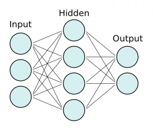
> We have to multiply each input node by a weight w and add a bias b.
> It is generally common to use a rectified linear unit (ReLU) for hidden layers, a sigmoid function for the output layer in a binary classification problem, or a softmax function for the output layer of multi-class classification problems.
### Keras
– Keras is a deep learning and neural networks API by Francois Chollet
$ pip3 install keras
kerasを使うにはbackgroundにtensorflowが動いていないといけないので、amazon linux2にtensorflowをインストールします。
$ pip3 install tensorflow
$ python3 -c “import tensorflow as tf; print(tf.reduce_sum(tf.random.normal([1000, 1000])))”
tf.Tensor(-784.01, shape=(), dtype=float32)
上手くインストールできたようです。
from keras.models import Sequential
from keras import layers

// 省略
input_dim = X_train.shape[1]

model = Sequential()
model.add(layers.Dense(10, input_dim=input_dim, activation='relu'))
model.add(layers.Dense(1, activation='sigmoid'))
model.add(layers.Dense(10, input_dim=input_dim, activation='relu'))
model.add(layers.Dense(1, activation='sigmoid'))

model.compile(loss='binary_crossentropy',
				optimizer='adam',
				metrics=['accuracy'])
print(model.summary())
$ python3 split.py
_________________________________________________________________
Layer (type) Output Shape Param #
=================================================================
dense (Dense) (None, 10) 17150
_________________________________________________________________
dense_1 (Dense) (None, 1) 11
=================================================================
Total params: 17,161
Trainable params: 17,161
Non-trainable params: 0
_________________________________________________________________
None
### batch size
history = model.fit(X_train, y_train,
					epochs=100,
					verbose=False,
					validation_data=(X_test, y_test)
					batch_size=10)
### evaluate accuracy
loss, accuracy = model.evaluate(X_train, y_train, verbose=False)
print("Training Accuracy: {:.4f}".format(accuracy))
loss, accuracy = model.evaluate(X_test, y_test, verbose=False)
print("Training Accuracy: {:.4f}".format(accuracy))
$ python3 split.py
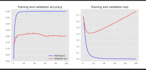
Training Accuracy: 1.0000
Training Accuracy: 0.8040
### matplotlib
$ pip3 install matplotlib
import matplotlib.pyplot as plt

// 省略
def plot_history(history):
    acc = history.history['accuracy']
    val_acc = history.history['val_accuracy']
    loss = history.history['loss']
    val_loss = history.history['val_loss']
    x = range(1, len(acc) + 1)

    plt.figure(figsize=(12, 5))
    plt.subplot(1, 2, 1)
    plt.plot(x, acc, 'b', label='Training acc')
    plt.plot(x, val_acc, 'r', label='Validation acc')
    plt.title('Training and validation accuracy')
    plt.legend()
    plt.subplot(1, 2, 2)
    plt.plot(x, loss, 'b', label='Training loss')
    plt.plot(x, val_loss, 'r', label='Validation loss')
    plt.title('Training and validation loss')
    plt.savefig("img.png")

plot_history(history)
おおお、なんか凄え