Category: Math

微分の関数とは

limb→a f(b)-f(a)/(b-a)

f(x)を微分するとf'(x)になる

(X^n)’ = nx^n-1
(sin x)’ = cos x
(tan x)’ = 1/cos^2x
(e^x)’ = e^x

うむ、微分の理論はなんとなくわかってきたか。

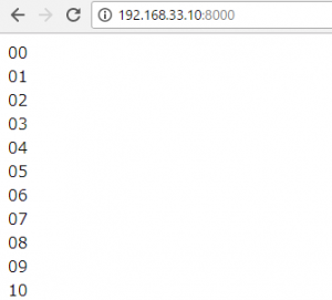
まず、00-99までは、for文を入れ子にして繰り返す。

for($i=0; $i<10; $i++){
	for($j=0; $j<10; $j++){
		echo $i.$j."<br>";
	}
}

000~999　入れ子を増やす

$time_start = microtime(true);
for($i=0; $i<10; $i++){
	for($j=0; $j<10; $j++){
		for($k=0; $k<10; $k++){
			echo $i.$j.$k."<br>";
		}		
	}
}
$time = microtime(true) - $time_start;
echo "{$time} 秒";

0.0011639595031738 秒

0～9999　4重にする

$time_start = microtime(true);
for($i=0; $i<10; $i++){
	for($j=0; $j<10; $j++){
		for($k=0; $k<10; $k++){
			for($l=0; $l<10; $l++){
				echo $i.$j.$k.$l."<br>";
			}		
		}		
	}
}
$time = microtime(true) - $time_start;
echo "{$time} 秒";

0.017668008804321 秒

なるほど

from decimal import Decimal, getcontext

from vector import vector
getcontext().prec = 30


class Line(object):
	NO_NONZERO_ELTS_FOUND_MSG = 'No nonzero element found'

	def __init__(self, normal_vector=None, constant_term=None):
		self.dimension = 2

		if not normal_vector:
			all_zeros = ['0']*self.dimension
			normal_vector = Vector(all_zeros)
		self.normal_vector = normal_vector

Ax + By + Cz = k1
Dx + Ey + Fz = k2
[A B C], [D E F] not parallel
dx = vector from x0 to x
Since x0, x in plane 1, dx is orth to n1

-One equation in two variables defines a line
-One equation in three variables define a plane

Caution: Count variables with coefficient 0
x + y = 2 defines a line in 2D
x + y = 2 defines a plane in 3D

systematically manipulate the system to make it easier to find the solution
– Manipulations should preserve the solution
– Manipulations should be reversible

Geometric object = a set of points satisfying a given relationship(e.g. equations)

“Flat” = defined by linear equations
Linear equations:
-Can add and subtract variables and constants
-Can multiply a variable by a constant

Linear: x + 2y = 1, y/2 – 2z =x
Nonlinear: x^2 -1 = y, y/x = 3

Equations come from observed or modeled relationships between real-world quantities.

ML for trading
stock:A, B
Wa = proportion of portfolio invested in A
Wb = proportion of portfolio invested in B
0 < Wa, Wb < 1 β value = measure of correlation of a stock's price movements with market movement β of portfolio = weighted average of individual components' β values Wa + Wb = 1 B portfolio = 2Wb - Wa = 0 Variables: weights of the stocks Constraints: equations representing physical realities or objectives Lines in Two dimensions Two pieces of info define a line -basepoint x -direction vector v x(t) = x + tv Ax + By = 0 (A and B not both 0)

Inner Products(Dot Products)
v*w = ||v||*||w||*cosΘ

def dot(self, v):
	return sum([x*y for x,y in zip(self.coordinates, v.coordinates)])

	def angle_with(self, v, in_degrees=False)
		try:
			u1 = self.normalized()
			u2 = v.normalized()
			angle_in_raddians = acos(u1.dot(u2))

			if in_degrees:
				degrees_per_radian = 180./ pi
				return angle_in_radians * degrees_per_radian
			else:
				return angle_in_radians

			except Exception as e:
				if str(e) == self.CANNOT_NORMALIZE_ZERO_VECTOR_MSG:
					raise Exception('Cannot compute an angle with the zero vector')
				else:
					raise e

P -> Q
magnitude of v = distance between P and Q
h^2 = (△x)^2 + (△y)^2
v = √(Vx^2 + Vy^2)

-A unit vector is a vector whose magnitude is 1.
-A vector’s direction can be represented by a unit vector.

Normalization: process of finding a unit vector in the same direction as a given vector.
[0 0 0] = 0
||0|| = 0
1 / ||0|| = ?

def magnitude(self):
	coordinates_squared = [x**2 for x in self.coordinates]
	return sqrt(sum(coordinates_squared))

def normalized(self):
	try:
		magnitude = self.magnitude()
		return self.times_scalar(1./magnitude)

	except ZeroDivisionError:
		raise Exception('Cannot normalize the zero vector')

def plus(self, v):
	new_coordinates = [x+y for x,y in zip(self.coordinates, v.coordinates)]
	return Vector(new_coordinates)

– Addition
– Subtraction
[1 3] – [5 1] = [-4 2]
– Scalar Multiplication
2, 1, 1/2, -3/2

[8.218 -9.341]+[-1.129 2.111]=[7.089 -7.23]
[7.119 8.215] – [-8.223 0.878]=[15.342 7.337]
7.41[1.671 -1.012 -0.318]= [12.382 -7.499 -2.356]

def plus(self, v):
	new_coordinates = [x+y for x,y in zip(self.coordinates, v.coordinates)]
	return Vector(new_coordinates)

def minus(self, v):
	new_coordinates = [x-y for x,y in zip(self.coordinates, v.coordinates)]
	return Vector(new_coordinates)

def times_scalar(self, c):
	new_coordinates = [c*x for x,y in zip(self.coordinates, v.coordinates)]
	return Vector(new_coordinates)

def __str__(self):
	return 'Vector: {}'.format(self.coordinates)

def __eg__(self, v):
	return self.coordinates == v.coordinates